gliderad2cp demo notebook
[1]:
from gliderad2cp import process_currents, process_shear, process_bias, tools, download_example_data
import cmocean.cm as cmo
import matplotlib.pyplot as plt
import xarray as xr
import numpy as np
Settings
There are several options that can be customised including:
QC correlation, amplitude and velocity thresholds
Velocity regridding options
Resolution of gridded output
Offsets to correct for transducer misalignment
These are all set in the options dict. The default options are a good place to start.
[2]:
options = tools.get_options(xaxis=1, yaxis=3, QC_correlation_threshold=80,
                            QC_amplitude_threshold=80, QC_velocity_threshold=1.5,
                            velocity_dependent_shear_bias_correction=False,
                            shear_bias_regression_depth_slice=(10,1000))
Available options are:
    correct_compass_calibration : [False, 'compass correction algorithm is awaiting publication and will be added upon acceptance. Contact Bastien Queste if you require.']
    shear_to_velocity_method : ['integrate']
    ADCP_mounting_direction : ['auto', 'top', 'bottom']
    QC_correlation_threshold : [80, 'minimum acceptable along-beam correlation value.']
    QC_amplitude_threshold : [80, 'maximum acceptable along-beam amplitude.']
    QC_velocity_threshold : [0.8, 'maximum acceptable along-beam velocity in m.s-1.']
    QC_SNR_threshold : [3, 'minimum acceptable dB above the noise floor.']
    velocity_regridding_distance_from_glider : ['auto', 'array of depth-offsets from the glider, in m, at which to interpolate beam velocities onto isobars to avoid shear-smearing. Negative for bottom-mounted ADCPs.']
    xaxis : [1, 'x-axis resolution in number of profiles of the final gridded products.']
    yaxis : [None, 'If None: ADCP cell size. If int: y-axis resolution in metres of the final gridded products.']
    weight_shear_bias_regression : [False, True, 'Give greater weight to dives with greater travel distance which can increase signal to noise.']
    velocity_dependent_shear_bias_correction : [False, True, 'Determine velocity dependent shear-bias correction coefficients rather than constant coefficients.']
    shear_bias_regression_depth_slice : [(0, 1000), 'A tuple containing the upper and lower depth limits over which to determine shear bias. Helpful to avoid increased noise due to surface variability. For deep diving gliders (500,1000) is good.']
    pitch_offset : [0, 'value to be added to pitch to correct for transducer-compass misalignment']
    roll_offset : [0, 'value to be added to roll to correct for transducer-compass misalignment']
    heading_offset : [0, 'value to be added to heading to correct for transducer-compass misalignment']
Default setting is the first value.
Options prefaced with a minus are not yet implemented.
Load data
gliderad2cp requires a netCDF file from a Nortek AD2CP which can be produced using the Nortek MIDAS software and a timeseries of glider data. This timeseries can be read from a netCDF, csv, or parquet file, or passed in as an xarray DataSet or pandas Dataframe. The essential variables are:
time
pressure
temperature
salinity
latitude
longitude
profile_number
There are several example datasets available from the function load_sample_dataset. We use one of the VOTO example datasets from the Baltic in this notebook
[3]:
data_file = download_example_data.load_sample_dataset(dataset_name="sea055_M82.nc")
adcp_file = download_example_data.load_sample_dataset(dataset_name="sea055_M82.ad2cp.00000.nc")
Step 1: calculate velocity shear
This is handled by the wrapper function process_shear.process(). The individual steps of processing are detailed in the documentation.
The output of this function is a gridded xarray dataset including data from the AD2CP like ensemble correlation and return amplitude, as well as calculated glider relative velocities and profiles of eastward, northward, and vertical velocities SH_E, Sh_N and Sh_U.
[4]:
ds_adcp = process_shear.process(adcp_file, data_file, options)
Loading glider data.
Loading ADCP data.
Merging glider data into ADCP dataset.
ADCP is bottom-mounted according to the accelerometer.
Performing sound speed correction.
    Corrected beam 1 velocity for sound speed.
    Corrected beam 2 velocity for sound speed.
    Corrected beam 3 velocity for sound speed.
    Corrected beam 4 velocity for sound speed.
Removing data exceeding correlation, amplitude and velocity thresholds.
    Beam 1 correlation: 40.06% removed
    Beam 1 amplitude: 19.95% removed
    Beam 1 velocity: 0.94% removed
    Beam 2 correlation: 42.13% removed
    Beam 2 amplitude: 24.32% removed
    Beam 2 velocity: 1.01% removed
    Beam 3 correlation: 44.22% removed
    Beam 3 amplitude: 25.10% removed
    Beam 3 velocity: 0.74% removed
    Beam 4 correlation: 41.98% removed
    Beam 4 amplitude: 23.28% removed
    Beam 4 velocity: 1.07% removed
Using the following depth offsets when regridding velocities onto isobars:
[ -0.  -1.  -2.  -3.  -4.  -5.  -6.  -7.  -8.  -9. -10. -11. -12. -13.
 -14. -15. -16. -17. -18. -19. -20. -21. -22. -23. -24. -25. -26. -27.
 -28. -29. -30. -31. -32. -33.]
    Regridding beam 1 onto isobars.
    Regridding beam 2 onto isobars.
    Regridding beam 3 onto isobars.
    Regridding beam 4 onto isobars.
Calculating X,Y,Z from isobaric 3-beam measurements.
Calculating E, N, U velocities from X, Y, Z velocities.
Calculating shear from velocities.
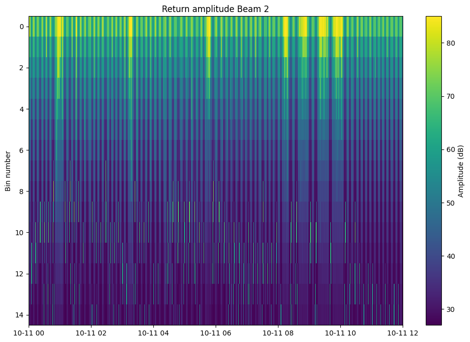
Plots
The output of process_shear.process() can be plotted to visually examine per-beam, per-bin values. This can be useful for fine tuning QC settings in options
[5]:
fig, ax = plt.subplots(figsize=(12, 8))
mappable = ax.pcolormesh(ds_adcp.time, ds_adcp.bin, ds_adcp.AmplitudeBeam2.T, cmap='viridis')#, vmin=0, vmax=100)
fig.colorbar(ax=ax,mappable=mappable, label='Amplitude (dB)')
ax.set(ylabel='Bin number', title='Return amplitude Beam 2', xlim=(np.datetime64("2024-10-11"), np.datetime64("2024-10-11T12")))
ax.invert_yaxis()
Step 2: shear to velocity
After calculating velocity shear, this can be integrated and referenced to estimate earth relative velocity profiles.
The function process_currents.process handles this step, returning DAC referenced velocity profiles.
Prerequisite: Get pre and post dive GPS locations from glider data
To calculate dive average current we require more variables, including estimates of the glider’s movement through the water. For this, we need the pre and post dive GPS locations of the glider. This calculation varies between glider models, processing tools and glider firmware versions. See the documentation for more examples of this calculation and make use of the verification plots. You can also provide your own input table of pre and post dive GPS locations and times.
[6]:
data = xr.open_dataset(data_file)
gps_predive = []
gps_postdive = []

dives = np.round(np.unique(data.dive_num))

_idx = np.arange(len(data.dead_reckoning.values))
dr  = np.sign(np.gradient(data.dead_reckoning.values))

for dn in dives:
    _gd = data.dive_num.values == dn
    if all(np.unique(dr[_gd]) == 0):
        continue

    _post = -dr.copy()
    _post[_post != 1] = np.nan
    _post[~_gd] = np.nan

    _pre = dr.copy()
    _pre[_pre != 1] = np.nan
    _pre[~_gd] = np.nan

    if any(np.isfinite(_post)):
        # The last -1 value is when deadreckoning is set to 0, ie. GPS fix. This is post-dive.
        last  = int(np.nanmax(_idx * _post))
        gps_postdive.append(np.array([data.time[last].values, data.longitude[last].values, data.latitude[last].values]))

    if any(np.isfinite(_pre)):
        # The first +1 value is when deadreckoning is set to 1, the index before that is the last GPS fix. This is pre-dive.
        first = int(np.nanmin(_idx * _pre))-1 # Note the -1 here.
        gps_predive.append(np.array([data.time[first].values, data.longitude[first].values, data.latitude[first].values]))

gps_predive = np.vstack(gps_predive)
gps_postdive = np.vstack(gps_postdive)
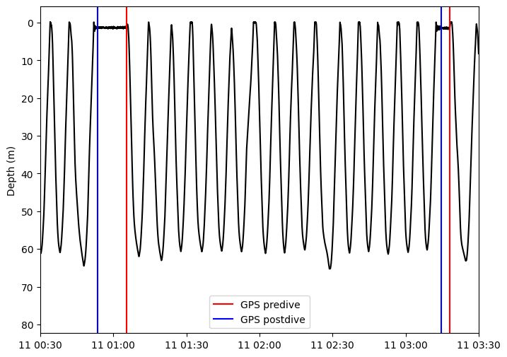
We expect gps_postdive and gps_predive to show as vertical blue and red lines respectively at the beginning and end of a glider surfacing manouvre. In a mission with multiple no-surface dives, as shown in the example below, the dives where the gliders does not surface to fix GPS, do not get assigned gps_postdive and gps_predive.
[7]:
fig, ax = plt.subplots(figsize=(8, 6))
ax.plot(data.time, data.depth, color='k')
for predive in gps_predive:
    ax.axvline(predive[0], color='r')
ax.axvline(predive[0], color='r', label='GPS predive')

for postdive in gps_postdive:
    ax.axvline(postdive[0], color='b')
ax.axvline(postdive[0], color='b', label='GPS postdive')
ax.invert_yaxis()
ax.set(xlim=(np.datetime64("2024-10-11T00:30"), np.datetime64("2024-10-11T03:30")), ylabel='Depth (m)')
ax.legend();
[8]:
currents, DAC = process_currents.process(ds_adcp, gps_predive, gps_postdive, options)
Calculating dive-averaged currents from dive and surfacing GPS coordinates.
Gridding shear data.
    Creating output structure and time-based metrics.
    Gridding flight metrics.
    Gridding eastward shear metrics.
    Gridding northward shear metrics.
    Calculating standard error as percentage of shear.
Calculating unreferenced velocity profiles from shear.
Referencing velocity profiles to dive-averaged currents using baroclinic velocity weighting.
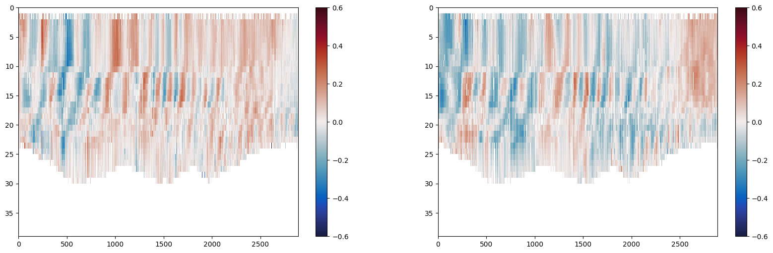
Plot DAC referenced currents
We can plot the output, DAC referenced eastward, northward, and upward velocities
[9]:
plt.figure(figsize=(20,6))

plt.subplot(121)
plt.pcolormesh(currents.velocity_E_DAC_reference, cmap=cmo.balance)
plt.gca().invert_yaxis()
plt.colorbar()
plt.clim([-0.6, 0.6])

plt.subplot(122)
plt.pcolormesh(currents.velocity_N_DAC_reference, cmap=cmo.balance)
plt.gca().invert_yaxis()
plt.colorbar()
plt.clim([-0.6, 0.6])
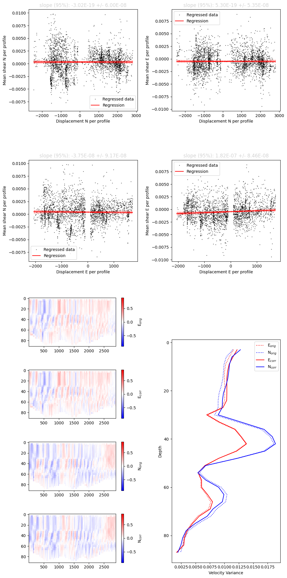
Step 3: Estimate and correct shear bias
This additional, optional processing step attempts to correct for along beam shear bias.
[10]:
currents = process_bias.process(currents,options)
Optimization terminated successfully.
         Current function value: 219.879552
         Iterations: 103
         Function evaluations: 195
Final results of shear bias regression:
    Along-glider bias :  -3.89E-03
    Across-glider bias : -9.79E-04

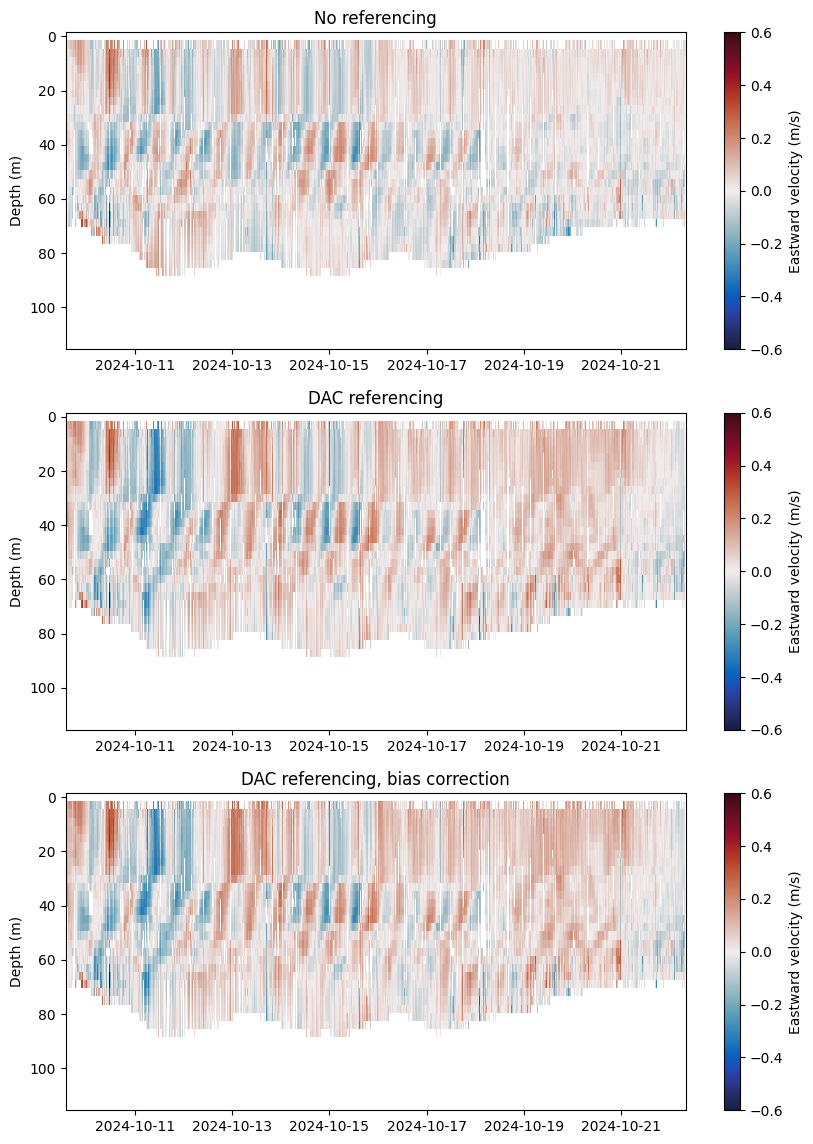
Compare outputs
The following three plots contrast the eastward velocities estimates at three crutical points of processing:
From integration of shear
After referencing integrated shear profiles to DAC
After applying the shear bias correction to DAC referenced velocities
[11]:
currents
[11]:
<xarray.Dataset> Size: 20MB
Dimensions:                                (depth: 39, profile_index: 2890)
Coordinates:
  * depth                                  (depth) float64 312B 0.0 ... 114.0
  * profile_index                          (profile_index) float64 23kB 1.0 ....
    time                                   (profile_index) datetime64[ns] 23kB ...
Data variables: (12/28)
    time_in_bin                            (depth, profile_index) float64 902kB ...
    heading_N                              (depth, profile_index) float64 902kB ...
    heading_E                              (depth, profile_index) float64 902kB ...
    speed_through_water                    (depth, profile_index) float64 902kB ...
    shear_E_mean                           (depth, profile_index) float64 902kB ...
    shear_E_median                         (depth, profile_index) float64 902kB ...
    ...                                     ...
    reference_N_from_DAC                   (profile_index) float64 23kB nan ....
    velocity_N_DAC_reference               (depth, profile_index) float64 902kB ...
    shear_bias_velocity_E                  (depth, profile_index) float64 902kB ...
    shear_bias_velocity_N                  (depth, profile_index) float64 902kB ...
    velocity_N_DAC_reference_sb_corrected  (depth, profile_index) float64 902kB ...
velocity_E_DAC_reference_sb_corrected (depth, profile_index) float64 902kB ...[12]:
variables = ["velocity_E_no_reference", "velocity_E_DAC_reference", "velocity_E_DAC_reference_sb_corrected"]
titles = ["No referencing", "DAC referencing", "DAC referencing, bias correction"]
fig, axs = plt.subplots(3, 1, figsize=(10,14))
for i in range(3):
    ax = axs[i]
    mappable = ax.pcolormesh(currents.time[:-1], currents.depth, currents[variables[i]][:, :-1], cmap=cmo.balance, vmin=-0.6, vmax=0.6)
    ax.invert_yaxis()
    fig.colorbar(ax=ax,mappable=mappable, label='Eastward velocity (m/s)')
    ax.set(ylabel='Depth (m)', title=titles[i])