gliderad2cp: Processing ad2cp data from gliders

gliderad2cp gliderad2cp processes data from the Nortek AD2CP acoustic doppler current profiler (ADCP) mounted on a glider. gliderad2cp takes data from the ADCP unit and the glider and combines them to produce estimates of vertical shear of velocity. It also provides functionality to integrate these velocity shear profiles into absolute earth relative water velocities.

Code hosted at https://github.com/bastienqueste/gliderad2cp

Package description

gliderad2cp estimates absolute ocean currents from glider ADCP data in several steps, each of which can be run independently and controlled via a dictionary of settings. gliderad2cp has three primary modules, each of which have a convenience wrapper function and a number of sub-funcitons

process_shear Calculate vertical shear of velocities from ADCP and glider data
process_currents Integrate shear profiles into relative velocities, referencing these to dive averace current.
process_bias Correcting velocity profiles for along-beam shear bias

Input

gliderad2cp requires two inputs:

A netCDF file from a Nortek AD2CP which can be produced using the Nortek MIDAS software
A timeseries of glider data. This timeseries can be read from a netCDF, csv, or parquet file, or passed in as an xarray DataSet or pandas Dataframe. The essential variables are:

time
pressure
temperature
salinity
latitude
longitude
profile_number

Example datasets are prodived via the function download_example_data.load_sample_dataset

A dictionary of processing options can be supplied. There are several options that can be customised including:

QC correlation, amplitude and velocity thresholds
Velocity regridding options
Resolution of gridded output
Offsets to correct for transducer misalignment

These are all set in the options dict returned by tools.get_options. If no options are passed, default values are used.

Step 1. Process shear

This is handled by the wrapper function process_shear.process((adcp_file_path, glider_file_path, options=None). The output of this function is a gridded xarray dataset including data from the AD2CP like ensemble correlation and return amplitude, as well as calculated glider relative velocities and profiles of eastward, northward, and vertical velocities SH_E, Sh_N and Sh_U.

process_shear.process() executes the following functions in order

load_data - load data from a Nortek AD2CP netCDF file and a glider data file or dataset
_velocity_soundspeed_correction - Corrects along beam velocity data for lack of salinity measurements in ADCP default soundspeed settings.
_quality_control_velocities - Removes bad velocity measurements based on velocity, amplitude and correlation criteria defined in options

The ADCP supplies observed relative velocities from an ensemble of pings. As well as the relative velocity, these ensembles have the amplitude response and inter-ping correlation. These velocities, amplitudes and correlations are used to quality control the input data. Using default settings, velocity estimates are discarded if they meet any of the following criteria:

Velocity > 0.8 m/s
Amplitude < 80 dB
Correlation < 80 %

These settings can be changed using the options dictionary.

Additionally the first X bins can be discarded at this stage if the operator has observed side-lobe interference.

_determine_velocity_measurement_depths - Determines what depth each velocity measurement was taken at for each beam, account for glider attitude
_regrid_beam_velocities_to_isobars - Regrids beam velocities onto isobars to avoid shear smearing in the final shear data

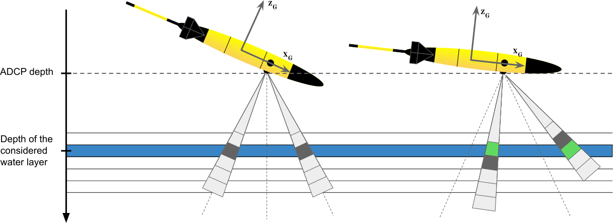
The Nortek AD2CP measurements are time-gated at the same intervals for each individual beam, meaning that the relation between echo delay and measurement range is the same for all 4 beams and does not account for the more open front and back beam angles. The purpose is to have 3 beams at equal angles from vertical when the glider is diving at the correct angle (17.4 ° from horizontal for the Nortek AD2CP; in grey on the left). If the glider is flying at a different angle, there will be a mismatch in depth between the 3 beams (in grey on the right) which requires regridding and use of different bins (in green on the right) to minimise shear smearing.

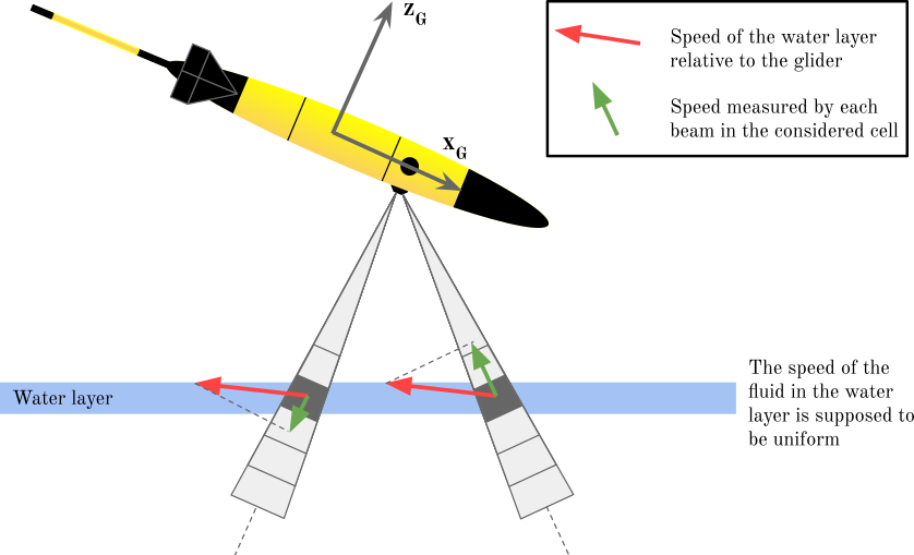
_rotate_BEAMS_to_XYZ - Coordinate transform that converts BEAM velocities to glider relative velocities X, Y, Z
_rotate_XYZ_to_ENU - Coordinate transform that converts velocity estimates relative to the glider (X, Y, Z) into the earth relative reference frame east, north, up (ENU)

Step 2. Process velocities

Prerequisite: Get pre and post dive GPS locations from glider data

To calculate dive average current we require more variables, including estimates of the glider’s movement through the water. For this, we need the pre and post dive GPS locations of the glider. This calculation varies between glider models, processing tools and glider firmware versions. See the documentation for more examples of this calculation and make use of the verification plots. You can also provide your own input table of pre and post dive GPS locations and times.

An worked example is provided in the notebook, showing GPS location calculation from a 2024 SeaExplorer dataset. More examples can be found in the section GPS calculations.

Vertical shear of horizontal velocities is calculated by gridded the ENU relative velocities into vertical bins. These vertical velocities of shear can then be integrated into velocity profiles.

process_currents.process() executes the following functions in order

get_DAC - Calculate dive-averaged currents using the ADCP as a DVL.

One source of absolute velocity estimate is the glider dive average current (DAC). Estimation of DAC depends on a flight model for the glider. Using speed through water from the ADCP, one can calculate the expected surfacing location of a glider from a known start position. The difference between this position and the actual surfacing location of the glider is caused by ocean currents, so the vertically averaged horizontal velocity can be estimated.

_grid_shear - Grid shear according to specifications (grid spacing etc.).

Vertical shear of horizontal velocities is calculated by gridded the ENU relative velocities into vertical bins. These vertical velocities of shear can then be integrated into velocity profiles.

_grid_velocity - Assemble shear measurements to reconstruct velocity profiles.

Profiles of velocity shear are integrated vertically to render vertical profiles of velocity. However, these vertical velocity profiles are relative and must be referenced to an absolute velocity

_reference_velocity - Reference vertical velocity profiles to dive-averaged currents, paying attention to the time spent at each depth.

The dive average current is used to reference the relative velocity profiles calculated in the previous step. Thus calculating earth relative absolute current velocities.

Step 3. Correct for shear bias

process_bias.process() executes the following functions in order

visualise - Produce collection of plots used to visalise estimated shear bias
regress_bias - Determine shear bias correction coefficients by empirically minimimising the slope of various linear regressions
correct_bias - Calculate the artificial velocity profile created by the shear bias and correct it in a new variable
visualise - Produce collection of plots used to visalise estimated shear bias after correction

All of these steps are demonstrated in the example notebook below.

GPS calculations

Example calculation for more recent SeaExplorer gliders (post 2023 firmware):

data = xr.open_dataset(data_file)
gps_predive = []
gps_postdive = []

dives = np.round(np.unique(data.dive_num))

_idx = np.arange(len(data.dead_reckoning.values))
dr  = np.sign(np.gradient(data.dead_reckoning.values))

for dn in dives:
   _gd = data.dive_num.values == dn
   if all(np.unique(dr[_gd]) == 0):
      continue

   _post = -dr.copy()
   _post[_post != 1] = np.nan
   _post[~_gd] = np.nan

   _pre = dr.copy()
   _pre[_pre != 1] = np.nan
   _pre[~_gd] = np.nan

   if any(np.isfinite(_post)):
      # The last -1 value is when deadreckoning is set to 0, ie. GPS fix. This is post-dive.
      last  = int(np.nanmax(_idx * _post))
      gps_postdive.append(np.array([data.time[last].values, data.longitude[last].values, data.latitude[last].values]))

   if any(np.isfinite(_pre)):
      # The first +1 value is when deadreckoning is set to 1, the index before that is the last GPS fix. This is pre-dive.
      first = int(np.nanmin(_idx * _pre))-1 # Note the -1 here.
      gps_predive.append(np.array([data.time[first].values, data.longitude[first].values, data.latitude[first].values]))

gps_predive = np.vstack(gps_predive)
gps_postdive = np.vstack(gps_postdive)

Example calculation for more older SeaExplorer gliders (post 2023 firmware):

gps_predive = []
gps_postdive = []

dives = np.round(np.unique(data.dive_num))

_idx = np.arange(len(data.dead_reckoning.values))
for dn in tqdm(dives):
    _dn = data.dive_num.values == dn
    _dr = data.dead_reckoning.values == 0
    _gd = (_dn & _dr).astype('float')
    _gd[_gd < 1] = np.NaN

    if all(np.isnan(_gd)):
        continue

    first = int(np.nanmin(_idx * _gd))
    last  = int(np.nanmax(_idx * _gd))

    gps_postdive.append(np.array([data.time.values[first], data.longitude.values[first], data.latitude.values[first]]))
    gps_predive.append(np.array([data.time.values[last], data.longitude.values[last], data.latitude.values[last]]))

gps_predive = np.vstack(gps_predive)
gps_postdive = np.vstack(gps_postdive)

Contents: